Image Details
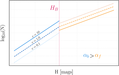
Caption: Figure A1.
Graphical representation of the differential power law. The “bright” end of the distribution (blue) is quantified by a slope αb, whereas the “faint” end (orange) is quantified by a slope αf (in this plot, αb > αf), with a break at HB. The size of the divot at HB is quantified by a contrast parameter c, that is the ratio of the differential binned objects predivot to the differential binned objects postdivot. For c = 1.0 (dashed), the power law reduces to a broken “knee” form, whereas for c < 1 and c > 1, a “divot” power law occurs, either increasing (dotted) or decreasing (solid) the number of objects postbreak, respectively.
Other Images in This Article
Copyright and Terms & Conditions
© 2026. The Author(s). Published by the American Astronomical Society.