Image Details
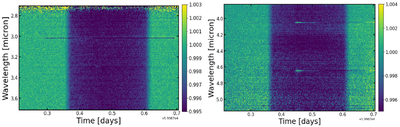
Caption: Figure 2.
Stacked detrended spectroscopic light curves (left NRS1, right NRS2) derived using the data-driven detrending approach described in Appendix C. First, the spectroscopic light curves were fitted using an empirical model (Equation (C1)). Following this, the second-order polynomial coefficients derived from the empirical model fit were smoothed in wavelength using a Gaussian kernel (Figure C2), and the smoothed coefficients were used to create a stellar variability model for each spectroscopic bin. The spectroscopic light curves were detrended using this variability model. The flare profile is derived from the best-fit flare parameters from the white light-curve fit, and the oscillation profiles are calculated by removing the stellar baseline model, transit, and flare profile from the white light curve (Figure C3). The detrending flare and oscillation profiles were scaled for each spectroscopic light curve, and the scaling factors were included as fitting parameters in the second iteration of the spectroscopic light-curve fits (Appendix C.2) to account for the wavelength dependence of the flare and oscillation amplitude. We can identify four outliers by eye on this diagram. These bins can be seen in this figure as horizontal stripes. We identify these bins at 3.03, 3.29, 4.04, and 4.65 μm and remove them from the subsequent analysis. From visual inspection of the light curves at these bins, we find that the temporal shapes of the flare/oscillations are different in these bins compared to the median profile used for detrending. Therefore, the data-driven detrending does not work well for these channels. The transit and the ingress/egress are visible by eye on the stacked detrended light curves. In the right panel, a darker patch is visible between 4.2 and 4.4 μm, which is due to CO2 absorption.
Other Images in This Article
Show More
Copyright and Terms & Conditions
© 2025. The Author(s). Published by the American Astronomical Society.