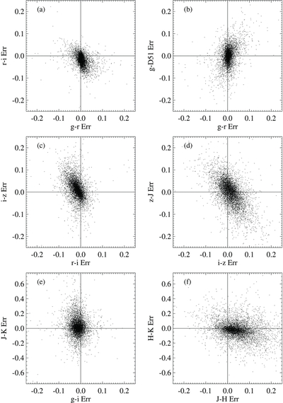
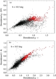
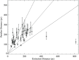
Comparison between observed and model colors. This plot represents all of the stars contained in one tile, covering an area spanning 1 deg in R.A. by 1 deg in decl. on the sky near galactic latitude b 10 5. Each point corresponds to one star, and the plotted positions show the residuals (in magnitudes) after subtracting the best-fit model from the photometry for that star, for two chosen colors (e.g., g− i vs. g− r, as in panel a). Different panels show various combinations of colors, indicated in the axis labels. The tile plotted here (at R.A. = 292° and decl. = +40°) is fairly typical of areas in which the model fits are good. There are several notable features. In panels (a) and (b), the rms scatter in the residuals is 0.02 mag or less in each of g− r, r− i, and g − D51. Errors are anticorrelated between g− r and g− i, but this tendency is more noticeable and has a different slope in the wings of the distributions than in the cores. 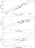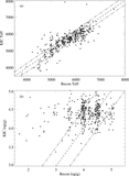In panels (c) and (d), note the larger scatter (especially in z− J), and also the strong negative correlations between these pairs of residuals. In panels (e) and (f), note the change in plot scale; the residuals in the IR colors are much larger than in the visible bands. The J− K and g− i residuals are almost uncorrelated, but one now sees a very significant offset from zero of the mean residual in g− i. The two IR colors in the bottom panel have only slightly correlated residuals, but the center of the J− H distribution is also far displaced from zero.