Image Details
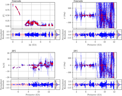
Caption: Figure 15.
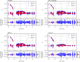
Representative examples of snapshot modeling results for both the Comrade (top row) and DPI (bottom row) pipelines. The top row of panels shows results from fitting an m = 4 mG-ring with Comrade to the HOPS low-band Sgr A* data on both April 6 and 7, while the bottom row of panels shows results from fitting an m = 2 mG-ring with DPI to the same data set. Each panel is arranged analogously to the individual panels of Figure 9, though the plotted data products are different. For the Comrade results, the visibility amplitudes and closure phases are used during fitting, so these are the data products shown in the top left and top right panels, respectively. For the DPI results, the log closure amplitudes and closure phases are used during fitting, so these are the data products shown in the bottom left and bottom right panels, respectively. All closure quantities are plotted as a function of the perimeter of the relevant polygon (i.e., triangles for closure phases, quadrangles for log closure amplitudes); the evident zero-valued closure phases and log closure amplitudes primarily correspond to so-called “trivial” polygons, i.e., those with near-zero area (M87* Paper III; Paper II). We note that the data-flagging procedures differ slightly between the two pipelines (see Sections 6.4.1 and 6.4.3), resulting in small differences in the fitted data sets.
Other Images in This Article
Show More
Copyright and Terms & Conditions
© 2022. The Author(s). Published by the American Astronomical Society.