

Image Details
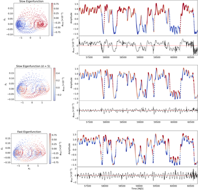
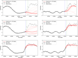
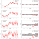
Caption: Figure 8.
4U 1705-44 light curve and phase space colored by eigenfunction amplitude. K was calculated with EDMD using a time-delay dictionary specified in Section 3.2 with length d = 50. The phase-space plots (left) show the flux xt against its time derivative ﹩{\dot{x}}_{t}﹩, computed with backward finite differences of the light curve. The lower panel of each group plots the eigenfunction values φ(t), with the dotted red line marking φ = 0. Top: slow-varying eigenfunction φslow(t); blue (φslow(t) < 0) and red (φslow(t) > 0) partition the light curve into low-flux and high-flux regimes, respectively. The light-curve plot shows color switching before the flux reaches large variance, demonstrating predictive ability. The phase-space plot (left) shows two distinct stable basins labeled by φslow, with low-flux (blue) on the left and high-flux (red) on the right; as in Figure 2, long “tails” of opposing color connect the basins, signifying color switching before the system begins switching to the opposite basin. We also overlaid the eigenfunction value plot (bottom right) with the light-curve flux at each point (light gray) to demonstrate how sign changes of φslow(t) tend to precede the flux changes visible in the light curve. Middle: φslow(t) from K calculated with time-delay length d = 5 observables. While state changes are predicted, false positives (color changes) are rampant during stable sections (right), with colors also changing during each stable oscillation. As a result, the phase-space plot (left) shows no labeling of stable regimes. Bottom: fast-varying mode φfast(t) oscillates rapidly within each oscillation. The phase-space plot also shows no clear regime labeling.
Other Images in This Article
Show More
Copyright and Terms & Conditions
© 2026. The Author(s). Published by the American Astronomical Society.

