

Image Details
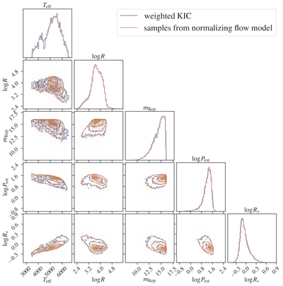
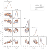
Caption: Figure 6.
One- and two-dimensional marginal distributions of ﹩({T}_{{\rm{eff}}},r,{m}_{{\rm{Kep}}},\mathrm{log}{P}_{{\rm{rot}}},\mathrm{log}{R}_{\star })﹩ for the KIC sample weighted by ﹩{\pi }_{{\rm{D}}| {\rm{TR}}}﹩ (blue) and for 60,000 samples drawn from the fitted normalizing-flow model (orange). The diagonal panels show the marginal distributions, and the off-diagonal panels show the joint contours. The contours enclose approximately 12%, 39%, 68%, and 86% of each distribution, corresponding to the default 0.5σ, 1σ, 1.5σ, and 2σ levels for a two-dimensional Gaussian distribution.
Other Images in This Article
Copyright and Terms & Conditions
© 2026. The Author(s). Published by the American Astronomical Society.

Copyright ©
2026 Astronomy Image Explorer. All Rights Reserved.
