Image Details
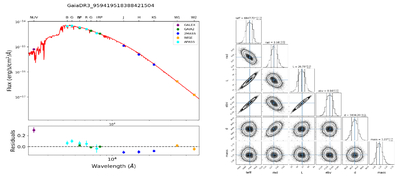
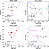
Caption: Figure 8.
Representative example of SED fitting for one of the identified variable stars. Left: observed photometric fluxes from multiple surveys are plotted along with the best-fit model (solid red line). The lower panel displays the corresponding residuals between the observed and model fluxes (in magnitudes). Right: corner plot illustrating the posterior probability distributions of the derived stellar parameters from the Markov Chain Monte Carlo analysis, including effective temperature (Teff), radius (R), luminosity (L), extinction (E(B − V)), distance (d), and mass (M). The contour levels denote the 1σ, 2σ, and 3σ confidence regions.
Other Images in This Article
Show More
Copyright and Terms & Conditions
© 2026. The Author(s). Published by the American Astronomical Society.