Image Details
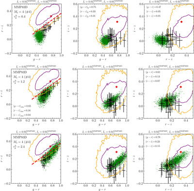
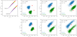
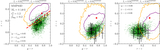
Caption: Figure 6.
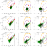
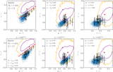
Color–color diagram variations as ﹩{\tau }_{g}^{{\rm{h}}}﹩ changes. The optical depths are set to 0.4, 1.2, and 2.4 in the top, middle, and bottom panels, respectively, with the Mach number fixed at Ms = 4. The ISRF model of MMP83D is assumed, with the i- and z-band intensities scaled down by a factor of 0.9 to match the r − i color. Green dots show the simulation results of scattered light, red diamonds indicate the colors of the incident ISRF, and black crosses mark the observational results of J. Román et al. (2020). Yellow and purple contours represent regions enclosing the 1σ and 2σ ranges of external galaxy samples from J. Román et al. (2020). The red dashed lines in the left panels (r − i versus g − r) denote the empirical relation used to distinguish cirrus clouds from extragalactic LSB features (J. Román et al. 2020). The initial colors of the input ISRF (MMP83D) are labeled with a subscript “0” in the top middle panel. Median values of the three simulated colors are shown in the right panels, while the mean observed colors are shown with a subscript “obs” in the middle-left panel. Note that the medians of the observed colors equal the means, except for the g − r color, whose median (0.62) is slightly smaller. The number (#4) in parentheses indicates the random sample index among the 10 realizations.
Other Images in This Article
Copyright and Terms & Conditions
© 2025. The Author(s). Published by the American Astronomical Society.