Image Details
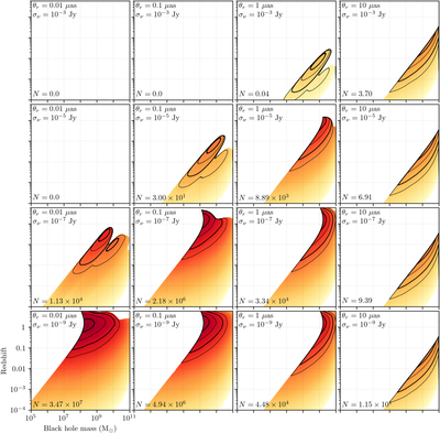
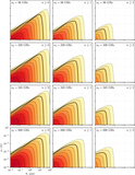
Caption: Figure 8.
The integrand from Equation (7), plotted logarithmically as ﹩\tfrac{{dN}}{d\mathrm{ln}(M)d\mathrm{ln}(z)}﹩, showing the distribution of the number of shadow-resolved and optically thin SMBHs that can be seen by a single baseline as a function of redshift and black hole mass. Each panel shows a different choice of θr and σν, and all panels assume an observing frequency of 230 GHz. The total number of black holes, integrated over M and z, is given in the lower left-hand corner of each panel. The color scale maps to the logarithm of the source number density (i.e., the number of sources per unit logarithmic interval in M and z), and the black contours enclose 50%, 90%, 99%, and 99.9% of the total source count. All panels share the same horizontal and vertical axis ranges, which are explicitly labeled in the bottom-left panel.
Other Images in This Article


Show More
Copyright and Terms & Conditions
© 2021. The Author(s). Published by the American Astronomical Society.