Image Details
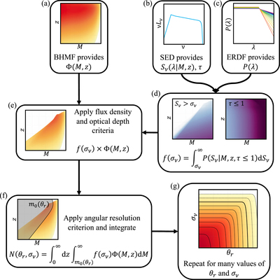
Caption: Figure 1.
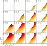
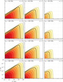
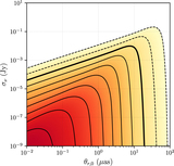
Flowchart illustrating the strategy for determining N(θr, σν) (see Section 2.1) using an example case of θr = 1 μas and σν = 10−5 Jy. Panels (a), (b), and (c) show the three primary inputs: the BHMF, the SED model, and the ERDF, respectively. The BHMF provides the global distribution of SMBHs as a function of M and z (see Section 2.2); the SED model predicts the emitted flux density and optical depth for every M, λ, and z (see Section 2.3); and the ERDF provides the distribution of Eddington ratios λ (see Section 2.4). In panel (d), the ERDF and the SED model are used to determine the fraction f(σν) of sources that simultaneously have flux densities exceeding σν (left plot in the panel) and are optically thin (i.e., τ < 1; right plot in the panel); in both plots, darker colors indicate a larger fraction. The combined fraction, as a function of M and z, is then used in panel (e) to modify the global SMBH distribution from the BHMF. In panel (f), we further apply the requirement that the angular shadow size exceed θr, which can be cast as a minimum mass m0(θr) at every z; N(θr, σν) is then determined by integrating over the region outside of the gray-shaded area. Finally, panel (g) illustrates that this procedure can be repeated for many other values of both θr and σν (see Section 2.5).
Other Images in This Article


Show More
Copyright and Terms & Conditions
© 2021. The Author(s). Published by the American Astronomical Society.