Image Details
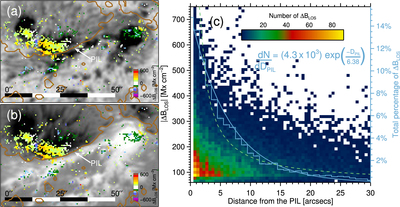
Caption: Figure 6.
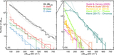
Relation between the PIL and ﹩{\rm{\Delta }}{B}_{\mathrm{LOS}}﹩. Left: location of ﹩{\rm{\Delta }}{B}_{\mathrm{LOS}}﹩ (color-coded pixels) and the PIL (brown line) during the X2.2—SOL2011-02-15T01:56 event. The continuum intensity image (panel a) and the magnetogram (panel b) during the maximum of the flare are shown in the background. The image scale is shown by the black and white dashed bar with a length of 50″ divided into four parts of 12.″5. ﹩{\rm{\Delta }}{B}_{\mathrm{LOS}}﹩ are clipped at ±600 Mx cm−2 according to the vertical color bar. Right: (c) plot showing the number and strength of ﹩{\rm{\Delta }}{B}_{\mathrm{LOS}}﹩ vs. distance to the PIL (﹩{D}_{\mathrm{PIL}}﹩). The color scale illustrates the number of ﹩{\rm{\Delta }}{B}_{\mathrm{LOS}}﹩ at a specific distance from the PIL. The histogram (light blue) shows the frequency distribution of ﹩{\rm{\Delta }}{B}_{\mathrm{LOS}}﹩ at certain distances from the PIL. The solid blue and dashed green lines show the best fit of an exponential and power-law model, respectively. A Kolmogorov–Smirnov test, which can be used as a goodness-of-fit test, showed that the frequency distribution ﹩{dN}/{{dD}}_{\mathrm{PIL}}﹩ more likely follows an exponential decay given by the equation in the plot.
Other Images in This Article
Copyright and Terms & Conditions
© 2018. The American Astronomical Society. All rights reserved.