

Image Details
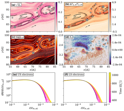
Caption: Figure 5.
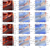
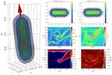
Top and middle rows: zoom-in onto a ﹩20\times 30\,{d}_{i}^{2}﹩ region inside the LS layer during the late nonlinear stage of the KHI (﹩t=778\,{{\rm{\Omega }}}_{c,i}^{-1}﹩). (a) Electron agyrotropy measure ﹩\sqrt{{Q}_{e}}﹩. (b) Normalized parallel electron temperature variation, ΔT∥,e/T∥,e0. (c) Logarithm of the out-of-plane electron current density, ﹩\mathrm{log}| {J}_{z,e}| ﹩. (d) Out-of-plane electric field, Ez. Black contours in panels (a) and (b) denote regions of intense electron current density, while white contours in panels (c) and (d) show magnetic flux isocontours. White crosses indicate magnetic X-points, while circled crosses indicate X-points with the largest values of ∣Ez∣, corresponding to the most active reconnection sites at the given time. (e, f) Temporal evolution of the normalized electron energy distributions in the US and LS layers, respectively. The black curve denotes the earliest distribution shown and serves as a reference for the progressive development of a suprathermal electron population during the nonlinear stage. Curves are colored according to time.
Other Images in This Article
Copyright and Terms & Conditions
© 2026. The Author(s). Published by the American Astronomical Society.

