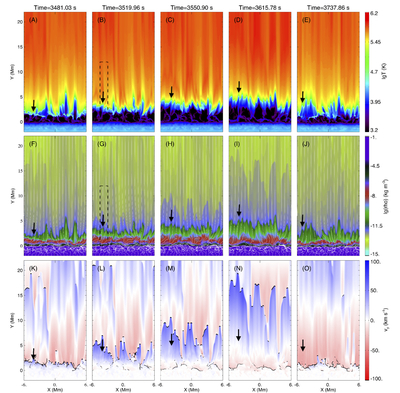
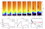
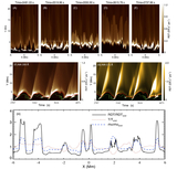
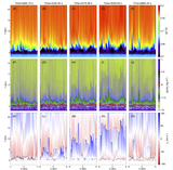
Evolution of spicules and the lower corona above them within a cycle of spicule formation in the 2.5D simulation with the initial magnetic field B₀ = 5 G. Distribution of logarithmic temperature (A)–(E), logarithmic density (F)–(J), and velocity in the Y-direction (K)–(O) at five different times are presented. The white solid curves in panels (F)–(J) outline the magnetic field lines. The black dashed boxes in panels (B) and (G) represent the zoomed-in region in Figures 6(A)–(H). The big, thick black arrow in each panel points to the top of one particular spicule with a temperature below 10⁵ K. The black contour lines in panels (K)–(O) outline the positions having large values of − ∇ · V, indicating the possible invoked slow-mode shocks. The animations of the corresponding temperature distribution, density distribution, and velocity (V_Y) distribution are available in the online journal.

(An animation of this figure is available in the online article.)

(An animation of this figure is available.)

The video/animation of this figure is available in the online journal.