Image Details
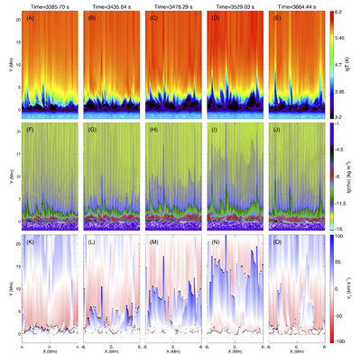
Caption: Figure 10.
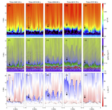
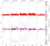
Evolution of spicules and the lower corona within a cycle of spicule formation in the higher resolution 2.5D run. All the initial and boundary conditions in this case are the same as those in the case with initial magnetic field B0 = B0y = 5 G shown in Figure 3. Distributions of logarithmic temperature (A)–(E), logarithmic density (F)–(J), and velocity in the Y-direction (K)–(O) at five different times are presented. The white solid curves in (F)–(J) are for the magnetic field lines. The black contour lines in (K)–(O) represent the regions having large values of − ∇ · V (shock fronts). The animations of the corresponding temperature distribution are available in the online journal.
(An animation of this figure is available in the online article.)
(An animation of this figure is available.)
The video/animation of this figure is available in the online journal.
Other Images in This Article
Show More
Copyright and Terms & Conditions
© 2026. The Author(s). Published by the American Astronomical Society.