Image Details
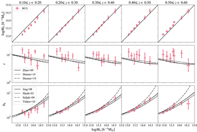
Caption: Figure 5.
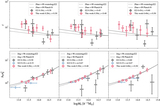
This plot shows the halo properties measured from the ESDs of our 35 lens samples. Shown in the different columns are the results for the lens samples in different redshift bins, as indicated at the top of each column. The x-axis is the halo mass measured from weak lensing. The data points in each panel show the best-fit values for the BCG centroid schemes. The panels in the top row show comparisons between the lensing halo mass (﹩\mathrm{log}{M}_{{\rm{h}}}﹩) and the group mass estimated using the abundance-matching method (﹩\mathrm{log}{M}_{{\rm{G}}}﹩). Note that the error along the y-axis is the standard error of the group mass of the sample, while the error along the x-axis indicates the 1σ confidence interval of the fitting. The black lines are reference lines where ﹩\mathrm{log}{M}_{{\rm{G}}}=\mathrm{log}{M}_{{\rm{h}}}﹩. The panels in the middle row show the concentration–mass relation measured from the ESDs. The y-axis is the halo concentration. The theoretical predictions of the c–M relations from Zhao et al. (2009), Dutton & Macció (2014), and Diemer & Joyce (2019) are shown as the solid, dashed, and dashed–dotted lines, respectively. The panels in the bottom row show the halo bias–mass relations. The theoretical predictions of the b–M relations from Jing et al. (1998), Sheth et al. (2001), Seljak & Warren (2004), and Tinker et al. (2010) are shown as the solid, dashed, dashed–dotted, and dotted lines, respectively.
Other Images in This Article
Copyright and Terms & Conditions
© 2022. The Author(s). Published by the American Astronomical Society.