Image Details
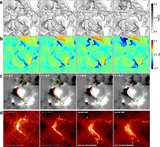
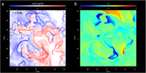
Caption: Figure 1.
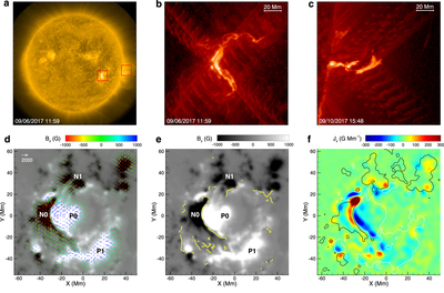
The flare location and photospheric magnetic field. (a) Full-disk image of the Sun observed with SDO/AIA 171 Å. The two boxes indicate the locations of the on-disk X9.3 flare on September 6 and the limb X8.2 flare that occurred on September 10. (b) and (c) SDO/AIA 304 Å images of the X9.3 flare and the X8.2 flare, respectively. (d)–(f) SDO/HMI vector magnetograms taken at 11:36 UT on September 6, which is 17 minutes before the onset of the X9.3 flare. In (d), the magnetic flux distribution, i.e., Bz, is overlaid by the transverse field vector (Bx, By) as denoted by the colored arrows. The main magnetic polarities P0, N0, P1, and N1 are labeled. In (e) the yellow curves are the locations of bald patches along the PIL. (f) Distribution of the vertical current density, which is defined as ﹩{J}_{z}={\partial }_{x}{B}_{y}-{\partial }_{y}{B}_{x}﹩. The contour lines are plotted for Bz = −500 G (colored black) and 500 G (white). The ratio of the direct current (DC) to the return current (RC) for the positive flux is ﹩| \mathrm{DC}/\mathrm{RC}{| }^{+}=2.31﹩, and for the negative flux it is ﹩| \mathrm{DC}/\mathrm{RC}{| }^{-}=2.26﹩.
Other Images in This Article

Show More
Copyright and Terms & Conditions
© 2018. The American Astronomical Society. All rights reserved.