Image Details
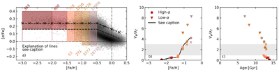
Caption: Figure 1.
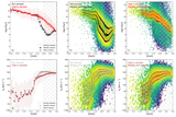
(a) [α/Fe] as a function of [Fe/H] for the full sample, with Gaia-Enceladus stars removed (see Section 2). The underlying data are shown as a 2D histogram with a power-law relationship. (This means that the colors are remapped onto a power-law relationship, y = xγ, where γ is the power, and if it is equal to 1, it simply gives the default normalization in Matplotlib.) The colored boxes define the different subsamples analyzed in panels (b) and (c). The number of stars in each bin is indicated in the figure. The dashed line shows Equation (1), which splits the data into high- and low-α stars, and the dashed line with crosses is the same line but raised by 0.08 dex. (b) The median Vϕ/σZ as a function of the median [Fe/H] for stars in each of the bins defined in panel (a). High- and low-α stars split by Equation (1) are indicated, and high-α stars resulting from the raised cut are shown by crosses. The solid line shows a smoothed fit to the underlying data. (c) The median Vϕ/σZ as a function of the median age for stars in each of the bins defined in panel (a). High- and low-α stars split by Equation (1) are indicated, and high-α stars resulting from the raised cut are shown by crosses. The gray shaded areas in panels (b) and (c) show the region 1 < Vϕ/σZ < 3; see discussion in Section 3.
Other Images in This Article
Copyright and Terms & Conditions
© 2026. The Author(s). Published by the American Astronomical Society.