Image Details
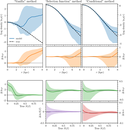
Caption: Figure 2.
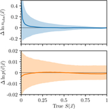
The gravitational densities (ρ = ∇2Φ/4πG) and their residuals (versus the true densities), as recovered by the three variants of Deep Potential. In all panels, the median value of the gravitational density is plotted, along with the shaded envelopes enclosing the 16th and 84th percentiles. It should be emphasized that the envelopes do not represent statistical uncertainty but rather the angular variation at surfaces of constant r or S(x). The percentiles are calculated over surfaces of constant distance from the origin, r (top two rows, subject to a cut on the true selection function: S(x) > 0.01) or S(x) (bottom two rows). Top row: ﹩\mathrm{ln}\rho ﹩ as a function of r. The dotted curves show the true density. Second row: residuals ﹩{\rm{\Delta }}\mathrm{ln}\rho =\mathrm{ln}{\rho }_{{\rm{model}}}-\mathrm{ln}{\rho }_{{\rm{true}}}﹩ as a function of r. Third row: residuals as a function of the true selection function ﹩S\left({\boldsymbol{x}}\right)﹩, illustrating the deterioration in the recovered density as the fraction of stars observed decreases. Bottom row: residuals in the selection function ﹩S\left({\boldsymbol{x}}\right)﹩ (as recovered by the “selection function” method) and true spatial density of tracers ﹩n\left({\boldsymbol{x}}\right)﹩ (as recovered by the “conditional” method), each as a function of the true ﹩S\left({\boldsymbol{x}}\right)﹩. In the top three rows, the vertical axes are the same for the “selection function” and “conditional” methods.
Other Images in This Article
Copyright and Terms & Conditions
© 2026. The Author(s). Published by the American Astronomical Society.