Image Details
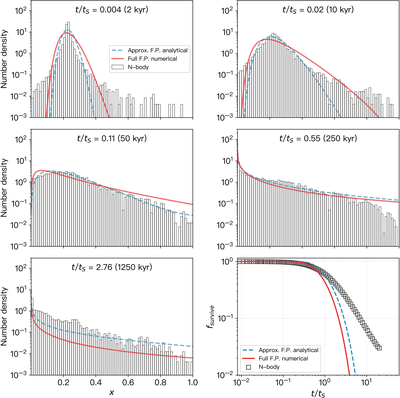
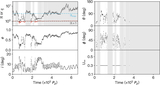
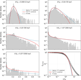
Caption: Figure 8.
Comparison of the particle energy distribution (x) at various times predicted by the Fokker–Planck equation (solid and dashed curves) and by direct numerical integrations (bar histograms). The blue curves show the analytical solution of the linearized (approximate) Fokker–Planck equation (Equation (49)), while the red curves correspond to the numerical solution of the full Fokker–Planck equation (Equation (46)). Particles are initialized with ﹩{{ \mathcal A }}_{0}=2.49﹩, e0 = 0.634, and i0 = 15﹩\mathop{.}\limits^{\unicode{x000b0}}﹩8, corresponding to U∞ = 0.5 or ﹩{ \mathcal T }=2.75﹩. The planet has mass Mp = 1 × 10⁻⁴ at ap = 1 au, and its scattering timescale tS = 450 kyr is computed using Equation (58). The final panel shows the surviving fraction fsurvive as a function of time, with the blue dashed curve given by Equation (51).
Other Images in This Article
Show More
Copyright and Terms & Conditions
© 2026. The Author(s). Published by the American Astronomical Society.