Image Details
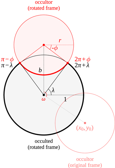
Caption: Figure 2.
Geometry of the occultation problem. The occulted body is centered at the origin and has unit radius, while the occultor is centered at ﹩({x}_{o},{y}_{o})﹩ and has radius r. The observer is located at ﹩z=\infty ﹩. We first rotate the two bodies about the origin through an angle ﹩\omega =\pi /2-\arctan 2({y}_{o},{x}_{o})﹩ so the problem is symmetric about the y-axis. In this frame, the occultor is located at ﹩(0,b)﹩, where ﹩b=\sqrt{{x}_{o}^{2}+{y}_{o}^{2}}﹩ is the impact parameter. The arc of the occultor that overlaps the occulted body (thick red curve) now extends from ﹩\pi -\phi ﹩ to ﹩2\pi +\phi ﹩, measured from the center of the occultor. The arc of the occulted body that is visible during the occultation (thick black curve) extends from ﹩\pi -\lambda ﹩ to ﹩2\pi +\lambda ﹩, measured from the origin. These are the curves along which the primitive integrals (Equations (31) and (32)) are evaluated. The angles ϕ and λ are given by Equations (24) and (25) and extend from ﹩-\pi /2﹩ to ﹩\pi /2﹩. When the occultor is completely within the disk of the occulted body, we define ϕ = λ = π/2 (Python).
Other Images in This Article

Show More
Copyright and Terms & Conditions
© 2019. The American Astronomical Society. All rights reserved.