Image Details
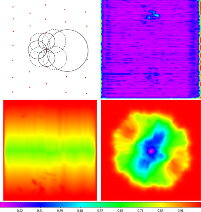
Caption: Figure 49.
Top left: from each data point, we “blow a bubble” in each of the coordinate system’s eight cardinal directions until it intersects another data point that is within 45° of the blow direction and that is more than a minimum angular distance away. We determine this minimum angular distance by taking all angular distances between consecutive measurements in the observation and performing outlier rejection on them, determining the minimum angular distance that is not rejected. (For daisies, the telescope’s slew speed is variable, with the smallest angular distances between consecutive measurements occurring at the ends/beginnings of scans, which is also where this is most difficult to measure accurately: the telescope’s rapid transition between deceleration and acceleration at the ends/beginnings of scans is often messy, resulting in data-point clustering. Consequently, we instead measure these angular distances at the center of each scan, where the telescope is moving fastest, with minimum acceleration/deceleration, and then divide by half of the number of scans, which gives what these angular distances should have been at the ends/beginnings of scans. We reject outliers as described in Sections 4–6 of Maples et al. (2018), using iterative bulk rejection followed by iterative individual rejection (using the mode + broken-line deviation technique, followed by the median + 68.3% value deviation technique, followed by the mean + standard deviation technique), using the smaller of the low and high one-sided deviation measurements. Data are weighted equally. In the case of appended mappings (Section 3.6.5), we adopt the minimum of each mapping’s minimum non-rejected angular distance in each overlap region.) Employing this minimum angular distance decreases computation time and prevents undersized bubbles from being blown, due to data-point clustering, usually at the ends/beginnings of scans, where the telescope changes direction. We take the largest bubble’s diameter as our local measure of θgap, from it calculate θw (Equation (14)), and then interpolate between these values at each pixel in the final image (footnote 28). Top right: raster example; resulting values of ﹩{\theta }_{w}=\min \{\tfrac{4}{3}\times {\theta }_{\mathrm{gap}},1\}﹩ for the 20 m horizontal raster from Figures 5, 23, and 38. Larger gaps are measured where the telescope’s momentum caused it to overshoot when changing directions, near the ends/beginnings of scans, and where the wind pushed the telescope across its direction of motion. Larger gaps are also measured where the RFI-subtraction algorithm removed data points, both due to RFI (e.g., the scan intersecting 3C 273) and in the outskirts of the beam pattern around Virgo A. Bottom left: nodding example; resulting values of ﹩{\theta }_{w}=\min \{\tfrac{4}{3}\times {\theta }_{\mathrm{gap}},1\}﹩ for the 40 ft nodding from Figure 26. This is a sparse mapping, with only ≈0.4 beamwidth gaps between scans at its middle decl., which, since this is a nodding pattern, yields gaps that are twice as large at the top and bottom of the mapping (Figure 2, middle panel). Bottom right: daisy example; resulting values of ﹩{\theta }_{w}=\min \{\tfrac{4}{3}\times {\theta }_{\mathrm{gap}},1\}﹩ for the 20 m daisy from Figures 25 and 44. The pattern is asymmetric, because gravity’s pull on the telescope resulted in narrower petals along the lower-left to upper-right diagonal, and wider petals orthogonally (see Figure 53).
Other Images in This Article


Show More
Copyright and Terms & Conditions
© 2019. The American Astronomical Society. All rights reserved.