Image Details
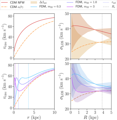
Caption: Figure 1.
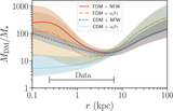
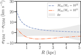
Illustration of mass models and their associated velocity dispersion profiles for different halo models described in Section 3.1. The top panels show CDM models with ﹩{\mathrm{log}}_{10}{M}_{200{\rm{c}}}/{M}_{\odot }=11﹩, ﹩{c}_{200{\rm{c}}}=10.5﹩, and rs = 9.3 kpc. The red solid line shows a cuspy NFW halo and the orange dotted–dashed line shows a cored αβγ halo. The bottom panels show FDM halos with an outer αβγ halo profile (plotted again for comparison) for a range of possible values of m22. The left-hand panels show the circular velocity profile associated to the halo, while the right-hand panels show the line-of-sight velocity dispersion profile. The range of orbital anisotropy values (from βani = −1 to 0.5) is shown by the shaded region, with the line indicating the isotropic (βani = 0) profile. Tangentially biased profiles (βani < 0) generally display velocity dispersion profiles that increase with radius, while radially biased profiles generally fall with radius. In the bottom left panel, the dotted lines show the expected soliton scale radius associated to each FDM halo (see Section 5.2). As the FDM scalar field mass gets larger, the profile approaches its CDM analog, with the deviations occurring on increasingly smaller scales. FDM is more “detectable” for lower m22 values where there is more mass in the soliton core. However, the projection of this mass profile into an observable velocity dispersion tends to wash out this signal (demonstrating the mass–anisotropy degeneracy). Furthermore even with a known anisotropy parameter, the FDM signal is degenerate with the inner DM slope (i.e., cored or cuspy).
Other Images in This Article
Copyright and Terms & Conditions
© 2019. The American Astronomical Society. All rights reserved.