Image Details
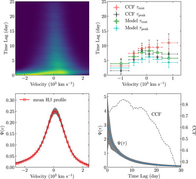
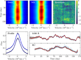
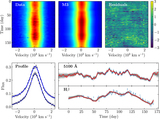
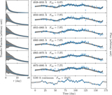
Caption: Figure 9.
Top left: an example of a transfer function obtained using model M3. Top right: comparison of velocity-binned time lags obtained from model M3 and CCF analysis. Bottom left: delay integral of the transfer function ﹩{\rm{\Psi }}(v)﹩, superposed on the observed, scaled mean Hβ profile. Shaded areas represent the 1σ error band. Bottom right: velocity integral of the transfer function ﹩{\rm{\Psi }}(\tau )﹩. Shaded areas represent the 1σ error band. The dashed line represents the CCF between the observed light curves of the continuum and Hβ fluxes.
Other Images in This Article
Show More
Copyright and Terms & Conditions
© 2018. The American Astronomical Society.
Copyright ©
2025 Astronomy Image Explorer. All Rights Reserved.