Image Details
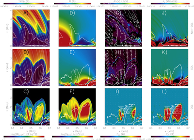
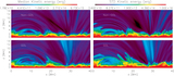
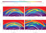
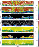
Caption: Figure 10.
Top row: maps of temperature (with magnetic field lines in white, panel (a)), density (panel (d)), divergence of the velocity (with velocity field as white arrows, panel (g)), and electric current density perpendicular to the plane (panel (j)) for the non-GOL simulations at t = 1240 s, snapshot = 328. Middle row: same as the top row, but for the GOL simulation (panels (b), (e), (h), and (k)) at t = 1350 s, snapshot = 340. Bottom row: Joule heating from the ambipolar diffusion (panel (c)), ambipolar diffusion (panel (f)), vertical Poynting flux due to the vertical ambipolar velocity (panel (i)), and the vertical Poynting flux due to the horizontal ambipolar velocity (panel (l)) for the GOL simulation. The ambipolar velocity field is shown with white arrows in panels (i) and (l). This region is a representative for magnetoacoustic shocks that go though the region between ﹩x=[25,45]﹩ Mm and ﹩x=[70,80]﹩ Mm, which does not show any dramatic reconnection. The white thick contours correspond to a 4000 K temperature.
Other Images in This Article
Show More
Copyright and Terms & Conditions
© 2017. The American Astronomical Society. All rights reserved.