Image Details
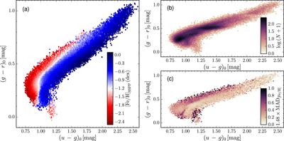
Caption: Figure 1.
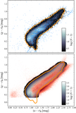
Summary of the training set shown in the ﹩{(u-g)}_{0},﹩ ﹩{(g-r)}_{0}﹩ CC diagram. Each plot shows summary statistics for the stars located within individual pixels, which are ≈0.01 mag on a side. Only pixels with ≥2 stars are shown. (a) The median [Fe/H] per pixel. Note that at constant ﹩{(g-r)}_{0}﹩ color, roughly corresponding to constant Teff, the ﹩{(u-g)}_{0}﹩ color provides an excellent diagnostic of [Fe/H]. (b) The total number of stars per pixel. Machine-learning methods typically perform best in regions where there is ample training data. The strong over-density with ﹩0.48\lt {(g-r)}_{0}\lt 0.55﹩ is due to the SDSS emphasis on targeting G stars, while the over-density at ≈ (0.9, 0.3) is due to the targeting emphasis on F-turnoff-like stars (see, e.g., Yanny et al. 2009). (c) The scatter in [Fe/H], as measured by 1.48 multiplied by the median absolute deviation (MAD), per pixel. Pixels with small scatter represent locations where the machine-learning model will be most accurate.
Other Images in This Article
Copyright and Terms & Conditions
© 2015. The American Astronomical Society. All rights reserved.