

Image Details
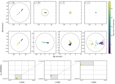
Caption: Figure 7.
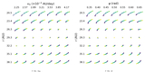
Example of the ε-cascade used to refine candidate links. Each column corresponds to one stage of the cascade, with the dashed circle indicating the current angular tolerance. Points are shown in projected (Δϕ, Δθ) coordinates and are colored by days since the first detection. As ε decreases from 30″ to 1″, the projected detections from a real object remain clustered while unrelated detections are rejected, producing a compact final candidate suitable for orbit fitting. The bottom row shows the two-dimensional (r, vΩ) cross section of the four-dimensional input grid at each refinement stage. The leftmost panel corresponds to the initial ε = 30″ bounds, subdivided to achieve a per-cell tolerance of ε = 10″. The cell containing the true spherical orbital elements of the implanted object (marked by the gold star) is highlighted in gray; the next panel zooms into that cell and subdivides it further, and the process repeats. We emphasize that the algorithm itself has no a priori knowledge of any true orbital elements and instead uses cluster tightness as its refinement metric, selecting the two cells with the smallest mean pairwise distance between projected detections. For reasons discussed below, this metric does not always select the cell containing the true orbital values. We present the cascade in this way to highlight the pattern of cluster convergence as the true values are approached.
Other Images in This Article
Show More
Copyright and Terms & Conditions
© 2026. The Author(s). Published by the American Astronomical Society.

