Image Details
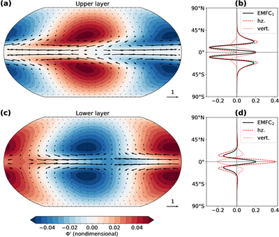
Caption: Figure 2.
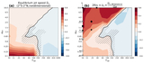
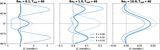
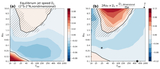
Numerical solution of the Matsuno–Gill problem (Equations (17a)–(17d)) with E = 0.02 and ﹩{ \mathcal S }{{\rm{Ro}}}_{T}{T}_{{\rm{rad}}}=1﹩, and its EMFC. (a) Upper-layer geopotential ﹩{{\rm{\Phi }}}_{1}^{{\prime} }﹩ (shading) and wind ﹩{{\boldsymbol{u}}}_{1}^{{\prime} }﹩ (arrows). (b) EMFC in the upper layer (solid), its horizontal convergence component (red dashed), and its vertical convergence component (red dotted line; see Equation (14), flux-form expression). (c, d) Same as panels (a) and (b), except for the lower layer.
Other Images in This Article
Show More
Copyright and Terms & Conditions
© 2026. The Author(s). Published by the American Astronomical Society.
Copyright ©
2026 Astronomy Image Explorer. All Rights Reserved.