

Image Details
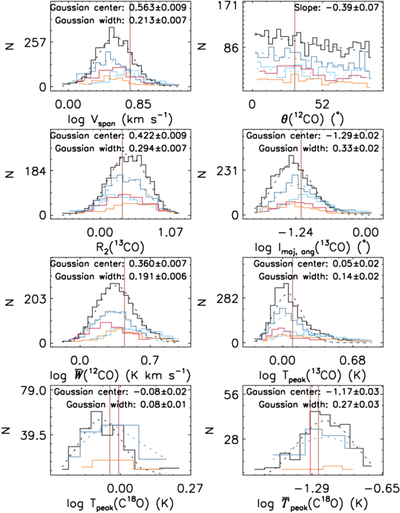
Caption: Figure 3.
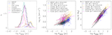
Distribution of observational parameters of identified MCs. We select eight observational parameters to show as examples. These parameters are Vspan, θ(12CO), R2(13CO), ﹩{l}_{\mathrm{maj},\mathrm{ang}}﹩(13CO), ﹩\overline{W}﹩(12CO), Tpeak(13CO), ﹩{T}_{\mathrm{peak}}({{\rm{C}}}^{18}{\rm{O)}}﹩, and ﹩\bar{T}{}_{\mathrm{peak}}{{\rm{(C}}}^{18}{\rm{O)}}﹩. The histograms for the overall MC sample without MCs possibly in the G120 spiral shock region are shown by black solid lines and are fitted with a Gaussian function, except for the oblique angle θ, which is fitted linearly. The fitting results are shown as black dashed lines. The Gaussian parameters and the slope of the fitted line are shown in the upper-right corner of each panel. For comparison, the histograms for MCs within the distance of 4 kpc and with significant C18O emission are shown by blue and light blue solid lines, respectively. These lines are multiplied by a factor of 2 for better visibility. These histograms are also fitted using the same methods as those used to fit the overall MC sample, and the corresponding fitting results are shown as blue and light blue dashed lines, respectively. The red solid lines show the histograms of the supra-Larson velocity dispersion MCs (i.e., those with velocity dispersions greater than 1.5 times the fitted σv–M relation). The histograms of MCs that are possibly in the G120 spiral shock region and in the G50 Perseus–Outer interarm spurs (i.e., the red crosses in Figure 8 of X. Zhou et al. 2025) are shown by the orange and brown solid lines, respectively. When there are insufficient MCs, only the mean value of the parameters is shown as a vertical line instead of a histogram. All parameter distributions and the corresponding fitted parameters are available in Science Data Bank at doi:10.57760/sciencedb.32354.
Other Images in This Article

Copyright and Terms & Conditions
© 2026. The Author(s). Published by the American Astronomical Society.

