

Image Details
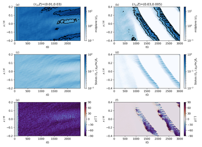
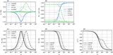
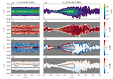
Caption: Figure 3.
Top panels: the x-axis profile of the midplane ϵ averaged along the y-axis plotted against time (the horizontal axis). The contours show 〈ϵ〉y = [1, 3, 10]. Middle panels: the x-axis profile of Stokes 〈I〉y, which is Stokes I averaged along the y-axis. Bottom panels: the corresponding χ also from Stokes Q and U averaged along the y-axis. The left and right columns correspond to the two simulations with (τs, Z) = (0.01, 0.03) and (0.03, 0.005), respectively. Note that the x-axis has a shear-periodic boundary condition.
Other Images in This Article
Copyright and Terms & Conditions
© 2026. The Author(s). Published by the American Astronomical Society.

Copyright ©
2026 Astronomy Image Explorer. All Rights Reserved.
