Image Details
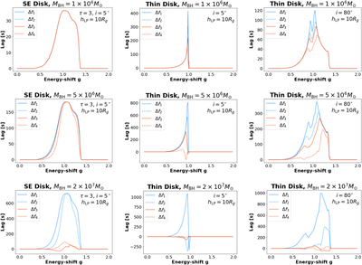
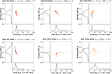
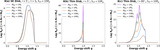
Caption: Figure 9.
We show explicitly how the lag–energy spectrum depends on the exact frequency band. Here, we use narrower frequency bands. The blue solid–dotted curves represent the narrow low-frequency bands of Δf1 = (0.8−1.6) × 10−4 Hz = (0.34–0.67) × 10−3 M6 c/Rg and Δf2 = (1.6−3.2) ×10−4 Hz = (0.67–1.34) × 10−3 M6 c/Rg, where M6 = MBH/106 M⊙. The red solid–dotted curves are for the narrow high-frequency bands Δf3 = (2−6) ×10−4 Hz = (0.84–2.52) × 10−3 M6 c/Rg and Δf4 = (6−10) × 10−4Hz = (2.52–4.20) × 10−3 M6 c/Rg. The three columns (left to right) represent different disk configurations: (a) the SE disk, (b) a low-inclination thin disk, and (c) a high-inclination thin disk. Each row has a different MBH = (1, 5, 20) × 106 M⊙. The most notable distinction between the two disk geometries is that the lag–energy spectrum of the SE disk remains almost the same despite the change in the frequency band until MBH becomes sufficiently large.
Other Images in This Article
Copyright and Terms & Conditions
© 2022. The Author(s). Published by the American Astronomical Society.