Image Details
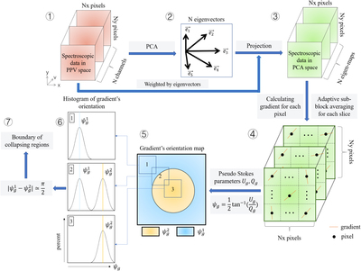
Caption: Figure 3.
Diagram of the VGT procedure to identify the gravitational collapsing regions (see Section 3). Steps 1 to 3 cover preprocessing of the spectroscopic data with dimensions Nx × Ny × N via PCA. Assuming that a PPV cube ρ(x, y, v) is a probability density function of three random variables x, y, v, we can construct a new orthogonal coordinate system formed by the eigenvectors (﹩{{\boldsymbol{e}}}_{1}﹩,﹩{{\boldsymbol{e}}}_{2}﹩ ... ﹩{{\boldsymbol{e}}}_{N}﹩) of PPV’s covariance matrix (see Equations (13) and (14)). By weighting the original PPV cube with the eigenvectors, we project the data into PCA’s eigenspace. In the new space, the significance of important eddies is separated and signified. Step 4 and step 5 consist of constructing the pixelized 2D gradients map (see Equations (16) and (17)). With the preprocessed data cube, we calculate the per pixel gradients in each slice through the convolution with Sobel kernels. Per pixel gradient slice then is processed by the per pixel adaptive sub-block averaging method (see Section 5.2), which takes the Gaussian fitting peak value of the gradient distribution in a selected sub-block to statistically define the mean magnetic field in the corresponding subregion. This step outputs an Nx × Ny × N gradient cube. Final 2D gradient’s orientation map results from the summation of the gradient cube, similarly to Stokes parameters (see Equation (17)). Step 6 and step 7 consist of identifying the boundary of gravitational collapsing regions through the double-peak algorithm (see Section 3.2). Based on theoretical considerations, gradients change their orientation by π/2 in gravitational collapsing regions. Therefore, in diffuse region 1, we can see the gradient’s histogram is approximately a single Gaussian distribution with the peak value located at ﹩{\psi }_{g}^{1}﹩. In gravitationally collapsing region 3, the peak value of the histogram becomes ﹩{\psi }_{g}^{2}﹩. However, in transitional region 2, the histogram appears bimodal, showing two peak values: ﹩{\psi }_{g}^{1}﹩ and ﹩{\psi }_{g}^{2}﹩. Corresponding pixel is labeled as the boundary of the collapsing regions once the difference between ﹩{\psi }_{g}^{1}﹩ and ﹩{\psi }_{g}^{2}﹩ is approximately π/2. Step 6 and step 7 can be achieved by the curvature algorithm (Section 3.3).
Other Images in This Article
Show More
Copyright and Terms & Conditions
© 2020. The American Astronomical Society. All rights reserved.