

Image Details
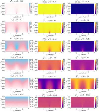
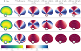
Caption: Figure 4.
Two-dimensional anisotropy angular distributions (for a slab where ﹩{\hat{{\boldsymbol{n}}}}_{{ \mathcal S }}\cdot \hat{{\boldsymbol{B}}}=0﹩) as a function of the cosine of the zenith angle, ﹩{\mu }_{kn}=\cos {\theta }_{kn}﹩, and the azimuthal angle ϕkB, of the intensity (Equation (38), left column), and the averaged electric field components ﹩| {\bar{{ \mathcal E }}}_{\parallel }^{2}| ﹩ (middle column) and ﹩| {\bar{{ \mathcal E }}}_{\perp }^{2}| ﹩ (right column), obtained in MAGTHOMSCATT. Rows correspond, from top to bottom, to ω/B = 0.01, 0.1, 0.25, 0.5, 2.0, and 100.0, spanning the strong field to effectively nonmagnetic scattering regimes discussed in Section 2.5. Note the varying normalization color scale for each row for HI.
Other Images in This Article
Show More
Copyright and Terms & Conditions
© 2026. The Author(s). Published by the American Astronomical Society.

