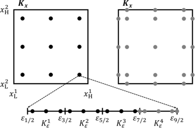
Illustration of key point sets of the nodal collocation DG scheme for the case with d_x = 2 for quadratic elements: N = k + 1 = 3. The left spatial element shows the LG spatial node set S_x (black dots). The right spatial element shows the spatial node set S_x (gray dots). An energy grid ﹩{{ \mathcal T }}_{\varepsilon }﹩ is attached to each spatial node x ∈ S_x, as illustrated below the spatial elements for the case with ﹩{\mathfrak{N}}=4﹩. For the first three elements, the LG node set ﹩{S}_{\varepsilon }^{{\mathfrak{e}}}﹩ (﹩{\mathfrak{e}}\in \{1,2,3\}﹩) is shown (black dots), while the node set ﹩{{\boldsymbol{S}}}_{\varepsilon }^{{\mathfrak{e}}}﹩ (﹩{\mathfrak{e}}=4﹩) is shown for the last element (gray dots). The point set ﹩{S}_{{\boldsymbol{z}}}^{{\mathfrak{e}}}={S}_{{\boldsymbol{x}}}\otimes {S}_{\varepsilon }^{{\mathfrak{e}}}﹩ is used to build the polynomial representation in Equation (75), while the polynomial representation is evaluated in the point set ﹩{{\boldsymbol{S}}}_{{\boldsymbol{z}}}^{{\mathfrak{e}}}={{\boldsymbol{S}}}_{\varepsilon }^{{\mathfrak{e}}}\otimes {{\boldsymbol{S}}}_{\varepsilon }^{{\mathfrak{e}}}﹩ for each element ﹩{{\boldsymbol{K}}}_{{\boldsymbol{z}}}^{{\mathfrak{e}}}﹩ in order to update the expansion coefficients in Equation (75) by the nodal collocation DG scheme.