Image Details
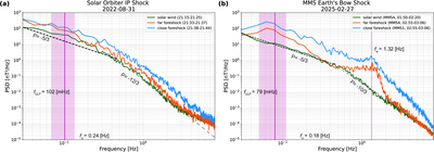
Caption: Figure 2.
A comparison of magnetic field PSDs in the foreshock of the IP shock and Earth’s bow shock in the spacecraft frame. For both panels, power-law slopes for different turbulent regimes are shown for reference, with stronger dissipation observed at the IP shock. Panel (a) shows PSD of the magnetic field from the Solar Orbiter spacecraft on 2022 August 31, upstream of the shock. Three distinct plasma environments are compared: the “close foreshock” immediately upstream of the shock (blue), a “far foreshock” region (orange), and a “solar wind” upstream interval representing the background solar wind (green). Characteristic frequencies, including the local ion cyclotron frequency (fci) and the expected ULF wave frequency (K. Takahashi et al. 1984), are indicated in the plot. Panel (b) shows a similar analysis for Earth’s bow shock on 2025 February 27, observed by the MMS mission. The plot compares the “close foreshock” (MMS1, blue) with the “far foreshock” (MMS4, orange) and a quiet upstream solar wind interval (MMS4, green). In addition to the fci and expected frequencies, the approximate location of the secondary peak associated with the presence of whistler waves is shown (fw ≈ 1 Hz). The shaded area for the expected ULF range is obtained by assuming an error of ±3 nT in upstream magnetic field and ±10∘ in the determination of θBn. The intervals used per line are also visualized as shaded areas in Figure 1.
Other Images in This Article
Copyright and Terms & Conditions
© 2026. The Author(s). Published by the American Astronomical Society.