Image Details
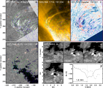
Caption: Figure 4.
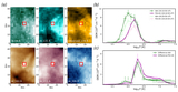
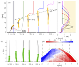
Correspondence between the magnetic fields, spicules, and EUV jet. (a) The Hα spicule trajectory readouts (green lines) from the GST/VIS −0.8 Å image are taken as a proxy for the magnetic field lines and copied to (b)–(d). (b) SDO/AIA 171 Å image with the LOS magnetogram (contours). (c) Same as (a) over the Dopplergram with the blue/red colors representing blueshift and redshift. The field lines are colored magenta in this panel. (d) An SDO/HMI LOS magnetogram with the contours at the levels of −40 G (blue) and +30 G (red). These contours are overplotted in panels (a)–(c) as well. (e) The three panels are GST/NIRIS LOS magnetic fields in the small FOV (cyan box in (d)) in units of arcseconds. (f) NIRIS magnetogram in the same FOV at another time in units of Mm. Two guide lines are the slits for scanning the 1D magnetic field distributions. (g) Distribution of the vertical magnetic field, Bz, read along the two slits. The animation shows panels (a) and (c) from 19:06:16 UT to 19:20:55 UT.
(An animation of this figure is available in the online article.)
(An animation of this figure is available.)
The video/animation of this figure is available in the online journal.
Other Images in This Article
Copyright and Terms & Conditions
© 2025. The Author(s). Published by the American Astronomical Society.