

Image Details
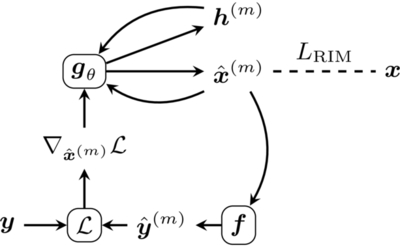
Caption: Figure 3.
Graphical representation of RIMs. A neural network gθ is trained to solve inverse problems by producing point estimates ﹩\hat{{\boldsymbol{x}}}﹩ of the model parameters x that produced an observation y through the forward model f. The neural network iteratively updates its predictions ﹩\hat{{\boldsymbol{x}}}﹩ using gradients of the negative log-likelihood function ﹩{ \mathcal L }\equiv -\mathrm{log}p({\boldsymbol{y}}| \hat{{\boldsymbol{x}}})﹩. The dashed line represents the loss function in Equation (15).
Other Images in This Article
Show More
Copyright and Terms & Conditions
© 2026. The Author(s). Published by the American Astronomical Society.

Copyright ©
2026 Astronomy Image Explorer. All Rights Reserved.
