

Image Details
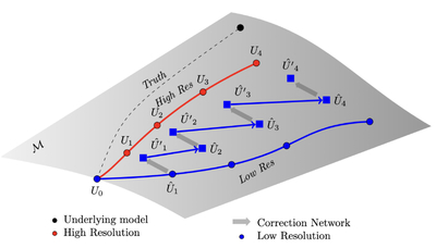
Caption: Figure 16.
Solver-in-the-loop: Schematic diagram showing how an integrated ML model can be used to correct a “low-resolution” simulation to recover the properties of a “high-resolution” simulation at significantly reduced computational cost. We visualize the evolution of the system as a path on the solution manifold ﹩{ \mathcal M }﹩, with each point representing a system state. The corrector network, ﹩{{ \mathcal B }}_{\theta }﹩, can be viewed as a geodesic flow on the manifold that pushes the low-resolution solution closer to either the reference high-resolution solution or the underlying truth (if suitable data are available). The augmentation network, ﹩{{ \mathcal B }}_{\theta }﹩ can be trained dynamically by running the low-resolution simulation to the end state, ﹩{\hat{U}}_{f}^{{\prime} }﹩ and then snapshots along the simulation can be compared with the reference simulation Ui. The derivatives of the loss can be used to update the parameters of the correction network, θ.
Other Images in This Article
Show More
Copyright and Terms & Conditions
© 2026. The Author(s). Published by the American Astronomical Society.

