

Image Details
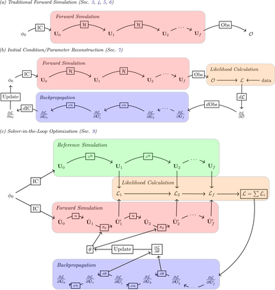
Caption: Figure 1.
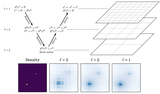
Schematic overview of forward and inverse workflows enabled by diffhydro. (a) Traditional simulation: an initial condition (IC) specified by parameters ϕ0 is mapped to the conservative state U0 and advanced forward through repeated applications of the hydrodynamic update operator ﹩{ \mathcal H }﹩, yielding a final state Uf from which observables ﹩{ \mathcal O }﹩ are computed. (b) Initial-condition/parameter reconstruction: the same forward model is paired with a likelihood ﹩{ \mathcal L }({ \mathcal O };{\rm{data}})﹩; automatic differentiation backpropagates gradients through the observable postprocessing map and each time step (dObs and ﹩d{ \mathcal H }﹩) to obtain ﹩\partial { \mathcal L }/\partial {{\boldsymbol{\phi }}}_{0}﹩, enabling gradient-based updates of ICs or physical parameters. (c) Solver-in-the-loop optimization: a reference simulation provides target states or observables at multiple times, defining a summed loss ﹩{ \mathcal L }={\sum }_{i}{{ \mathcal L }}_{i}﹩. A differentiable forward run ﹩\hat{{\boldsymbol{U}}}﹩ is controlled by trainable parameters θ (e.g., closure/source-term models ﹩{{ \mathcal B }}_{}\theta ﹩); gradients ﹩\partial { \mathcal L }/\partial {\boldsymbol{\theta }}﹩ are obtained by backpropagating through both ﹩{ \mathcal H }﹩ and ﹩{{ \mathcal B }}_{}\theta ﹩, allowing for optimization of embedded models while preserving the underlying finite-volume numerics.
Other Images in This Article
Show More
Copyright and Terms & Conditions
© 2026. The Author(s). Published by the American Astronomical Society.

