Image Details
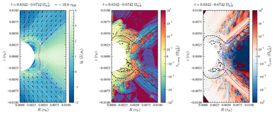
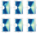
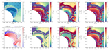
Caption: Figure 8.
Time-averaged properties from ﹩t=0.6342\,{{\rm{\Omega }}}_{{\rm{KH}}}^{-1}﹩ to ﹩0.6742\,{{\rm{\Omega }}}_{{\rm{KH}}}^{-1}﹩ for simulation G101Dn5In4n3. Panel (a) shows the density distribution (color scale), poloidal velocity field (black arrows), and magnetic field lines (solid white lines). The scale of the poloidal velocity is shown at the top right of the panel, and the magnetic field lines are depicted by the contours of the time-averaged poloidal magnetic flux at several specific levels. Panel (b) presents ﹩{\bar{\tau }}_{a,{\rm{mag}}}﹩ (color scale) superposed with streamlines of ﹩-R\overline{{B}_{\phi }{{\boldsymbol{B}}}_{{\rm{pol}}}}﹩, while panel (c) illustrates the distribution of ﹩{\bar{\tau }}_{a,{\rm{dyn}}}﹩. Both panels utilize symmetrical logarithmic color scales, with the range from −10−3 to 10−3 shown in linear scale while the other parts in logarithmic scale. In both panels (b) and (c), black dashed lines indicate the contours of the critical density ﹩{\rho }_{{\rm{crit}}}=100\,{\rho }_{{\rm{\inf }}}﹩, aiding in the identification of the disk profile. Violet dashed lines in panels (a)–(c) mark the boundaries where the azimuthal velocity reaches 80% of the Keplerian velocity (where ﹩\overline{{v}_{\phi }}=0.8\sqrt{G{M}_{{\rm{pl}}}/r}﹩). For reference, the escape velocity and the Keplerian timescale at the planetary radius (rpl = 0.0027 rH) are vesc = 27vKH and ﹩{{\rm{\Omega }}}_{{\rm{K}}}^{-1}=1.4\times 1{0}^{-4}\,{{\rm{\Omega }}}_{{\rm{KH}}}^{-1}﹩, respectively.
Other Images in This Article
Show More
Copyright and Terms & Conditions
© 2026. The Author(s). Published by the American Astronomical Society.