Image Details
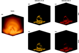
Caption: Figure 1.
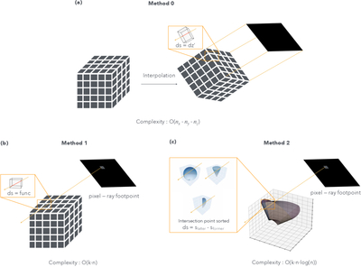
Schematic diagrams of different methods. Panel (a) illustrates the basic logic of Method 0. Before performing radiation synthesis for each selected perspective, the grid data must be interpolated into another grid orthogonal to the selected perspective to ensure that ds in each cell is constant. The complexity of this method is consistently ﹩{ \mathcal O }(N)﹩. Panel (b) illustrates the basic logic of Method 1, applicable to both Cartesian and spherical coordinate systems. Each pixel in the image represents the footpoint of a ray. Along each ray, the value of ds passing through each cell is dynamically calculated, and the radiative transfer equation solution is integrated. For spherical coordinate systems, the data must first be interpolated into Cartesian coordinates before applying Method 1. Panel (c) presents Method 2 for solving the radiation transfer equation directly in spherical coordinates. Unlike Method 1, Method 2 directly computes the intersection points between rays and spherical coordinate planes, followed by filtering and sorting. This approach preserves all resolution without any loss. Due to the unavoidable sorting operation, its complexity is ﹩{ \mathcal O }(k\cdot n\cdot \mathrm{log}n)﹩.
Other Images in This Article
Copyright and Terms & Conditions
© 2026. The Author(s). Published by the American Astronomical Society.