

Image Details
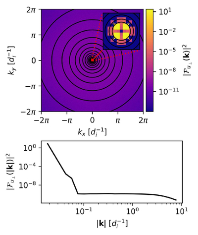
Caption: Figure 2.
An illustrative example of how spatial spectra are computed in this work. Top: a 2D Fourier transform of the benchmark ﹩{ \mathcal M }=16﹩ simulation’s initial u⊥ field (the left panel of Figure 1). The color of each pixel represents the power in the corresponding wave mode with k = (kx, ky). The black circles represent the bin edges used to compute the 1D spectrum shown in the bottom panel. The red square shows the size of the area highlighted in the inset panel. The inset panel shows the lowest wavenumbers. Bottom: a 1D representation of the above 2D Fourier spectrum. Each point in this spectrum is the mean value of the pixels in between each black circle in the top panel.
Other Images in This Article
Show More
Copyright and Terms & Conditions
© 2026. The Author(s). Published by the American Astronomical Society.

