Image Details
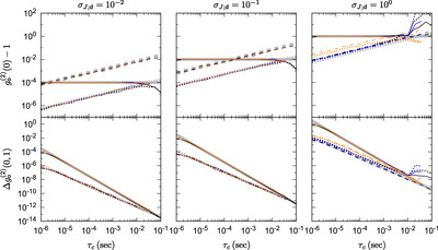
Caption: Figure 4.
Numerical results in simulations of slow variability. In the simulations, photometry is taken at a cadence of 1 ms for 216 samples, and the coherence time of the background variability is within the plotted range. On top is plotted the mean value of ﹩{\hat{g}}_{{\mathsf{o}}}^{(2)}(0)-1﹩ (solid) as well as the standard deviation in ﹩{\bar{g}}_{{\mathsf{o}}}^{(2)}(0)﹩ (dashed) and ﹩{\hat{g}}_{{\mathsf{o}}}^{(2)}(0)﹩ (dotted) over one hundred trials. Note the divergence in the error in ﹩{\bar{g}}_{{\mathsf{o}}}^{(2)}﹩ and ﹩{\hat{g}}_{{\mathsf{o}}}^{(2)}﹩ as ﹩{\sigma }_{J;{\mathsf{d}}}﹩ shrinks. On bottom is the mean value of ﹩{\rm{\Delta }}{\hat{g}}_{{\mathsf{o}}}^{(2)}(0,1)﹩ (solid) and the standard deviations of ﹩{\rm{\Delta }}{\bar{g}}_{{\mathsf{o}}}^{(2)}(0,1)﹩ (dashed) and ﹩{\rm{\Delta }}{\hat{g}}_{{\mathsf{o}}}^{(2)}(0,1)﹩ (dotted). Three models of noise are considered: a scintillation power spectrum with Gaussian fluctuations (blue) and lognormally distributed intensity (orange), and Gaussian fluctuations with a Gaussian-shaped g(2)(t) function (black). These are compared to theoretical expectations (thick, light-gray lines).
Other Images in This Article
Copyright and Terms & Conditions
© 2025. The Author(s). Published by the American Astronomical Society.