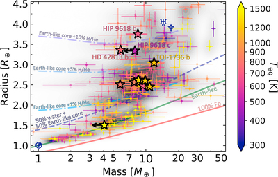
The mass–radius diagram for small planets. Data comes from the NASA Exoplanet Archive’s planetary systems table, as accessed on 2022 November 17 (NASA Exoplanet Archive 2022). Planets with mass and radius measurements to better than 50% and 15% fractional precision, respectively, are shown as the circles with 1σ error bars. The opacity of the points is proportional to mass measurement precision (i.e., a less-precise mass measurement translates to a more transparent marker). Color corresponds to equilibrium temperature assuming zero Bond albedo and full day–night heat redistribution. Underlying contours come from Gaussian kernel density estimation of the confirmed planets described above. The 11 transiting planets from this work are overplotted as the stars. Mass upper limits (98% confidence) are plotted for HD 25463 c (yellow star near the radius valley) and HIP 9618 c (labeled). A handful of composition curves are plotted for reference (Lopez & Fortney 2014; Zeng et al. 2016, 2019). The curves of H/He envelopes atop Earth-like cores come from Lopez & Fortney (2014) and are chosen for a planet receiving 10× Earth’s incident flux (i.e., T _eq ≈ 500 K) orbiting a 10 Gyr-old, solar-metallicity star. The 50% water plus 50% Earth-like composition curve from Zeng et al. (2019) is calculated for a fixed temperature of 700 K at 100 bar, which determines the planetary model’s specific entropy. Note that familiar features of the planet radius distribution are now visible as two-dimensional features in the mass–radius plane. These include the radius valley (Fulton et al. 2017; Van Eylen et al. 2018), with center near 6 M _⊕ and 1.8 R _⊕, and the radius cliff (e.g., Kite et al. 2019), as seen by in the steep drop-off in the number of planets around 3 R _⊕.