Image Details
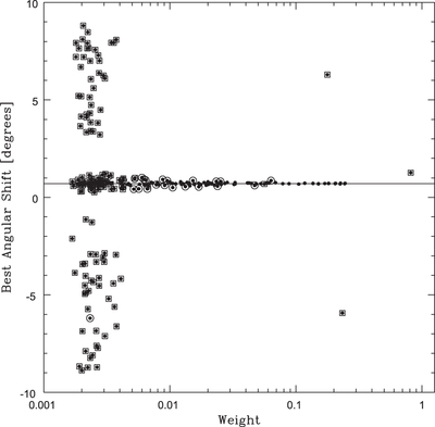
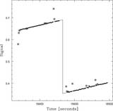
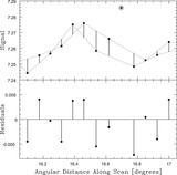
Caption: Figure 28.
Best angular shift between adjacent scans vs. cross-correlation weight for all scans in a 20 m observation. Many of the low-weight best angular shifts are not well defined, because their corresponding scans are noise dominated. A few of the high-weight best angular shifts are incorrect, due to RFI contamination (consequently, simply taking the weighted mean of these values would yield a poor result). To eliminate both cases, for each best angular shift, we calculate the probability that it could, by chance alone, be as close as it is to both its preceding and following values, and eliminate all best angular shifts for which this probability exceeds one-half divided by the best angular shift sample size (e.g., Chauvenet 1863; Maples et al. 2018; squared points). (For two, adjacent, best angular shifts, δi and δi+1, it is not difficult to show that this probability is given by ﹩{p}_{i,i+1}=\tfrac{| {\delta }_{i+1}-{\delta }_{i}| }{{\rm{\Delta }}}\left(2-\tfrac{| {\delta }_{i+1}-{\delta }_{i}| }{{\rm{\Delta }}}\right)﹩, where Δ is the angular length of the scans. For three, this probability is given by ﹩2{p}_{i-1,i}{p}_{i,i+1}﹩.) The remaining best angular shifts repeat consistently for at least three consecutive measurements, and consequently are likely due to astronomical signal, not noise or RFI contamination. We take the unweighted mean of these values (line), robust-Chauvenet-rejecting any remaining outliers (circled points). (We reject outliers as described in Sections 4–6 of Maples et al. 2018 using iterative bulk rejection followed by iterative individual rejection (using the mode + broken-line deviation technique, followed by the median + 68.3% value deviation technique, followed by the mean + standard deviation technique), using the smaller of the low and high one-sided deviation measurements. Data are weighted equally, in case any of the remaining high-weight data are still biased by RFI contamination (or by source saturation, as is the case in Figure 26).)
Other Images in This Article

Show More
Copyright and Terms & Conditions
© 2019. The American Astronomical Society. All rights reserved.