Image Details
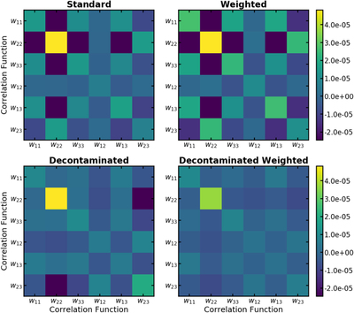
Caption: Figure 10.
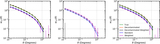
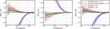
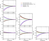
Estimator covariances across redshift bins for the case with three target redshift bins of Section 5.2 for an example theta bin (with θ = 0.°79 as the nominal center of the bin in log(θ)); these probe the covariances in the estimators without accounting for LSS sample variance. Here, wαβ refers to the CF between galaxies in redshift bins α and β, and as noted in the text, we estimate the estimator covariance as ﹩\left\langle \left\{{\widehat{w}}_{i}({\theta }_{k})-{w}_{i}^{\mathrm{true}}({\theta }_{k})\right\}\left\{{\widehat{w}}_{j}({\theta }_{k})-{w}_{j}^{\mathrm{true}}({\theta }_{k})\right\}\right\rangle ﹩ for each estimator, where i, j run over all the correlations (both auto and cross) and the expectation value is over all the realizations. Note that this is not sensitive to sample variance, since the true CF for each realization is subtracted from the observed CF for that realization. The left column shows estimator covariances in contaminated samples constructed using photo-z point estimates before (top) and after (bottom) decontamination, while the right column shows the estimator covariances in CF estimates using our Weighted estimator before (top) and after (left) decontamination. We see that our new decontaminated estimators reduce the covariances, with Decontaminated Weighted outperforming Decontaminated.
Other Images in This Article
Show More
Copyright and Terms & Conditions
© 2020. The American Astronomical Society. All rights reserved.