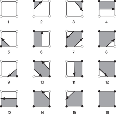
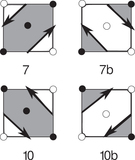
Marching-squares algorithm. Each set of four adjacent pixels for the discretized field δ_ij can take one of 16 possible combinations of “in” or “out” states. Black circles denote points in our grid for which the density lies inside the excursion set δ_ij > σ₀ν, and white circles are “out” points with δ_ij < σ₀ν. We label each case with an integer 1 ≤ N_c ≤ 16. Between each “in” and “out” state, we linearly interpolate between corners of the box to find the point along the edge of the square that satisfies δ = σ₀ν. We then connect these vertices, shown as solid black arrows. The arrow defines the boundary of the excursion region and is directed such that it always flows anticlockwise around the “in” states. The cases N_c = 7 and N_c = 10 are ambiguous, as discussed in the text.