Image Details

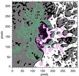
Caption: Figure 4.
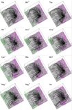
Images showing the magnitude of the current density | J | after integrating vertically through the computational domain for most of the models presented in Figure 2. Algorithms using the same class of method tend to produce similar patterns, as evident in the top row (showing models produced using optimization algorithms) and in the middle two rows (showing models produced using Grad–Rubin-style current-field iteration algorithms). The bottom row illustrates three different versions of the Valori magnetofrictional model, illustrating some of the effects associated with the process of embedding vector magnetogram data into line-of-sight magnetogram data to produce lower-boundary data. Shown are the Val model of Figure 2 which weights more heavily the boundary data inside the Hinode/SOT–SP field of view, a model for which the lower-boundary data were weighted uniformly, and a smaller-domain model encapsulating only the volume overlying the Hinode/SOT–SP field of view. The integrated current map from the Am2 − model in Figure 2 is almost identical to that of the Am1 − model, and is not shown.
Other Images in This Article
Copyright and Terms & Conditions
© 2009. The American Astronomical Society. All rights reserved.