

Image Details
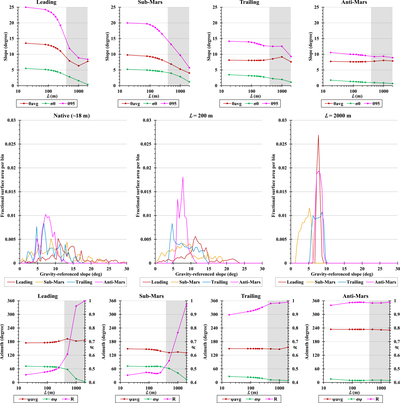
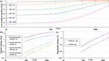
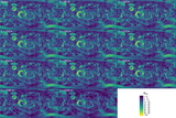
Caption: Figure 5.
Scale responses in the four representative 2° × 2° equatorial regions (one column per region in the top and bottom rows). Top row, as functions of the smoothing wavelength: area-weighted mean slope ﹩{\theta }_{{\rm{avg}}}﹩, slope standard deviation ﹩{\sigma }_{\theta }﹩, and 95th-percentile slope ﹩{\theta }_{95}﹩. Middle row: area-weighted slope-frequency distributions of the four regions for the native model and L = 200 and 2000 m. Bottom row, likewise as functions of the smoothing wavelength: circular mean azimuth ﹩{\psi }_{{\rm{avg}}}﹩, circular standard deviation ﹩{\sigma }_{\psi }﹩, and mean resultant length ﹩R﹩. Fixed facet assignments are defined in Section 2.1. In the top and bottom rows, the shaded band marks ﹩{\boldsymbol{L}}﹩ greater than 386.8 m, the approximate equatorial width of a 2° window: within it, the e-fold smoothing wavelength exceeds the spatial support over which the statistics are computed, so the plotted values describe the within-window continuation of the globally smoothed field rather than a regional response resolved at that wavelength. They are shown for completeness. The middle row is not shaded because its abscissa is slope angle rather than ﹩{\boldsymbol{L}}﹩.
Other Images in This Article

Copyright and Terms & Conditions
© 2026. The Author(s). Published by the American Astronomical Society.

