Image Details
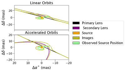
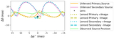
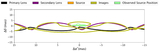
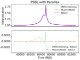
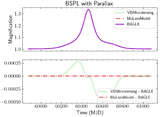
Caption: Figure 5.
Source and lens trajectories for linear (upper panel) and accelerated (lower panel) approximations of orbital motion of binary lenses. The solid black line is the primary lens, the solid purple line is the secondary lens, and the solid yellow lines are the image positions. The green line is the flux-weighted average of the lensed source position, as observed on the sky. Note that magS = 16. In both panels, the source is stationary; the primary lens has a proper motion of μL,⊙ = [−3.76 mas yr−1, −3.76 mas yr−1]; the secondary lens has a proper motion of ﹩{{\boldsymbol{\mu }}}_{{L}_{s},\odot }﹩ = [−2.76 mas yr−1, −2.76 mas yr−1]. For our model with acceleration, we provide the following input for aLrel,⊙ = [1 mas yr−1, −1 mas yr−1]. In both cases, the Einstein time is tE,⊙ = 412 days, the Einstein radius is 6 mas,and u0,⊙ = 0.5. Note that this scenario does not involve a caustic crossing, and thus it produces only three images.
Other Images in This Article
Show More
Copyright and Terms & Conditions
© 2026. The Author(s). Published by the American Astronomical Society.