Image Details
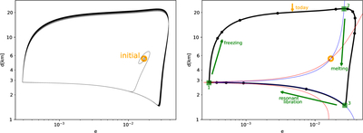
Caption: Figure 3.
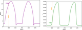
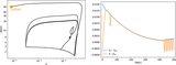
Numerical evolution in the e–d plane. Left panel: The black curve displays the system’s evolution, after it is initialized at the global equilibrium point. It escapes from equilibrium, and then traces out repeating limit cycles. Right panel: The black curve is the same as in the left panel, but restricted to the limit cycle. The black circles on the curve are separated by 1 Myr, over the course of one cycle. The blue and red curves are the equilibrium heating and cooling curves, repeated from Figure 2, with the blue showing H = C and the red showing H = Heq.
Other Images in This Article
Copyright and Terms & Conditions
© 2025. The Author(s). Published by the American Astronomical Society.
Copyright ©
2026 Astronomy Image Explorer. All Rights Reserved.